Many of us have written a monte carlo raytracer. One of the key results is that the results are extremely noisy, and are usually distributed as white noise in screen space. In order to mitigate this, the usual convention is to increase the number of samples per pixel in order to make the image converge to ground truth. This, however, isn’t really possible for real-time applications like games which usually have a target of 16ms per frame. In such scenarios, the scene is usually rendered with one sample per pixel(spp) and usually a spatio-temporal denoiser is used to filter out the noise.

However, what if I told you there was a way to significantly improve the perceptual quality of low spp images without making any changes whatsoever in to your raytracer? And what if I also told you that the entire implementation, at least for the first pass, can fit into a compute shader with less than 100 lines of code? Sounds great right!? Well it is! This method was first described in [1] by Eric Heitz and Laurent Belcout in 2019, and in this blog post I’ll hopefully describe a way that you can integrate in your raytracer without much trouble. This blog post is a result of over a week of work by me in collaboration with Alan Wolfe @Atrix256 who helped me a lot to understand some of the more theoretical aspects of the paper.

Background and Original Paper

First, let’s talk about the theory. If you instead only care about the implementation of the sorting pass then click here. So the goal is distribute the errors of Monte Carlo integration as blue noise in screen space. I’ll first talk about the theoretical model as described in section 3 of [1] and then a simple implementation of idea using a temporal implementation described in section 4 of [1].

Theory and formulation

As decribed in [1], this is an a posteriori formulation, that is, we have information from the previous frame and we will use it to improve the next frame. Now, consider a conventional Monte Carlo raytracer where each pixel uses a seed that is used to generate the random variables that are used to spawn ray directions from a specified position, in order to get diffuse and specular reflections on the entities. For diffuse you might use a random number to sample a random direction in a cosine weighted hemisphere oriented about the normal of the point. For specular, you might want to sample a random direction from the specular lobe, which is usually determined by the microfacet distribution of the object (see [2] for a great explanation of these concepts in more detail).

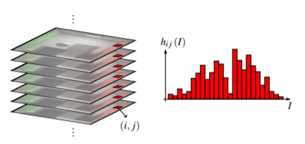
This image, taken from [1], describes the histrogram of estimates of a pixel rendered across different frames. If we render the scene multiple times with a different seed each frame, the result of of the Monte Carlo estimate of the rendering integral will be different each frame. And the bar graph shown above is the Histogram of Estimates, that is, the statistical representation of all the values that the pixel can take. And thus the value h_ij on the y axis of the graph is the Probability density function over the space of pixel estimates [1]. Now here is where the paper gets a little confusing so I will do my best to explain it in as simple terms as possible. For each pixel, rendering it means to compute a seed and use to generate random variables to spawn the rays. The result of spawning these rays is a value I_ij for a pixel that is random each frame, and you thus see a white noise pattern on the scene. Now instead what if we chose our seeds in such a way that if we sample the random values I_ij (as seen in the graph) from the distribution h_ij, in such a way that instead of getting a uniform random distribution for ‘I_ij’ we get correlated random numbers, such as those present in blue noise. To do this we will use a blue noise texture for random number generation and then map it to a random I_ij from the ditribution h_ij in order to get correlated errors. By doing this we a essentially distributing the errors in such a way that they look like blue noise in screen space and not the usual white noise.

Temporal Implementation of the Theory

Since the above theoretical model is very expensive, and the cost of rendering multiple previous frames in order to get the next frame is prohibitively expensive, especially for video games, [1] Essentially describes a temporal method which uses the previous rendered frame in order to improve the next frame by looking at the neighborhood pixels. In practice this algorithm creates permutations to the pixel seeds between two frames such that the errors become distributed as blue noise. The target dithering tile also changes each frame which is necessary for temporal filtering algorithms. In this part I will only describe the first part of their algorithm called the “Sorting Pass”.

Sorting Pass

A sampling property, as described by [1] is that using inverse transform sampling on a set of discrete 1 dimensional data is equivalent to sampling a list of the sorted data. Since the values I_ij of a pixel (i,j) is discrete, the inverse transform sampling can be done by sorting the set and getting a random index. In practice, this pass requires you to collecting the rendered value of the neighboring pixels, sorting them, and then sampling from the sorted list. In order to reduce the cost of getting the neighboring pixels for each pixel, we amortize it by processing blocks of BxB size together. The dithering tile is changed each frame for the temporal filtering algorithms as described above. In practice, I used the same blue noise texture just offset using Robert’s R2 low discrepancy sequence [3].

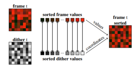
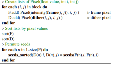
This figure illustrates the algorithm as described in section 4.1 of [1]. You essentially divide both the previous frame and the blue noise texture to blocks of size B x B. For each block you sort the pixels, in case of the frame you can sort it by its luma value, in case of the blue noise texture, you can sort by the pixel’s greyscale value. Once the sorting is done, you have a 1 to 1 mapping between the pixel values and the blue noise values. The pixel values are mapped with respect to their quantities they represent in their respective blocks. This mapping results in a permutation that is applied to the pixel seeds. In the above figure the permutation is applied to the frame values, in practice, this is only applied on the pixel seeds. The algorithm is very simple and can be implemented in less then 100 lines of code. You can see the appendix below to see my compute shader that implements it. But in pseudocode form here it is.

Results

Here is a result of what this technique looked like in my rendering engine:

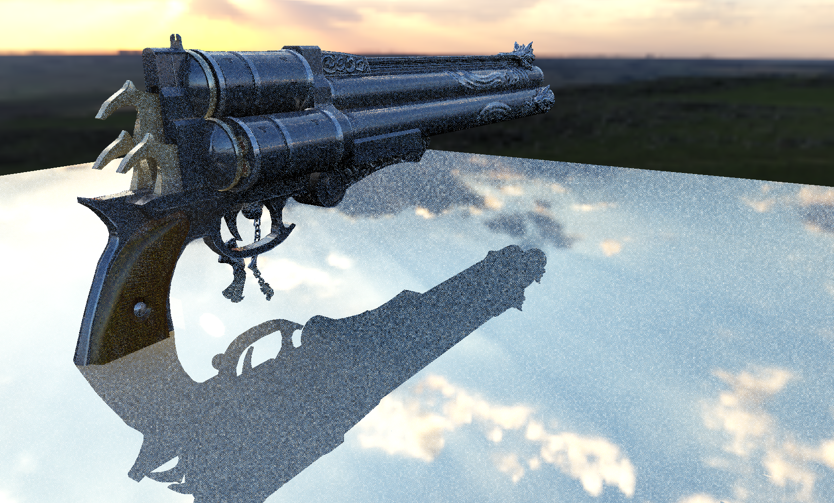This scene was rendered using my own D3D12 + DXR rendering engine. I used a block size of 4

This is the result of converting white noise to blue noise using my implementation of the algorithm

Limitations

As you might have noticed from the renders above, there are block artifacts in all of these images. These are caused due to the fact that we are processing the pixels in blocks instead of the whole image at once which means that the results will vary from block to block. Another limitation is that since we have a different noise pattern for each frame, we are going to see a different blue-noise dithering mask, and if we change the blue noise each frame, the blue noise quality gathered in the previous frame is lost.

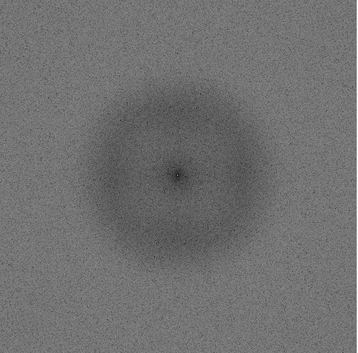
This DFT shows that the blue noise generated with just the sorting pass isn’t perfectly blue as some low frequency details are clearly present. This can be mitigated using a method called the ‘Retargeting Pass’ as described by Heitz and Belcour, but that is the topic for part 2 -mostly because at the time of writing I haven’t implemented it yet :).

References

1. The initial paper that described this method
2. Great Resource on Importance Sampling
3. The R2 Sequence

Appendix - Implementation using Compute Shaders

My primary purpose on trying this algorithm was to test its efficacy and potential usability in video games, since that is my main area of interest. As promised here is my compute shader that calculates the seeds for the next frame right after the previous frame has rendered. You can also look at it here as I would update it as I implement more changes.

groupshared uint newRandSeeds[BLOCK * BLOCK];
groupshared float3 colors[BLOCK * BLOCK];
groupshared float3 blueNoiseColors[BLOCK * BLOCK];
groupshared uint randSeeds[BLOCK * BLOCK];

[numthreads(BLOCK, BLOCK, 1)]
void main(uint3 groupID : SV_GroupID, // 3D index of the thread group in the dispatch.
uint3 groupThreadID : SV_GroupThreadID, // 3D index of local thread ID in a thread group.
uint3 dispatchThreadID : SV_DispatchThreadID, // 3D index of global thread ID in the dispatch.
uint groupIndex : SV_GroupIndex)
{
    
    float2 offset = GenerateR2Sequence(frameNum);
        
    uint initialSeed = InitSeed2(dispatchThreadID, 1920);
    randSeeds[groupIndex] = initialSeed;
    
    if(frameNum == 0)
    {
        newSequences[(dispatchThreadID.y) * 1920 + (dispatchThreadID.x)] = initialSeed;
        return;

    }

    randSeeds[groupIndex] = newSequences[(dispatchThreadID.y) * 1920 + (dispatchThreadID.x)];
    
    colors[groupIndex] = float3(CalcIntensity(prevFrame.Load(float3(dispatchThreadID.xy, 0)).rgb), groupThreadID.x, groupThreadID.y);

    uint samplePosX = (dispatchThreadID.x + offset.x*512) % 512;
    uint samplePosY = (dispatchThreadID.y + offset.y*512) % 512;
    blueNoiseColors[groupIndex] = float3(blueNoise.Load(float3(samplePosX, samplePosY, 0)).r, dispatchThreadID.x, dispatchThreadID.y);
    
    
    GroupMemoryBarrierWithGroupSync();

    if (groupIndex == 0)
    {
        Sort(colors);
        Sort(blueNoiseColors);
    }
    
    GroupMemoryBarrierWithGroupSync();

    uint outIndex = blueNoiseColors[groupIndex].z * 1920 + blueNoiseColors[groupIndex].y;
    uint currentIndex = colors[groupIndex].z * BLOCK + colors[groupIndex].y;
    
    newSequences[outIndex] = randSeeds[currentIndex];

}