Real time raytracing has become very popular in the last year or so, especially with the release of current generation of consoles which has made it more accessible to people. Even then, raytracing in real time is far slower than rasterization and we are only able to afford very few samples per pixel. This leads to very noisy results, which usually requires a spatio temporal denoising pass. One such domain which can produce noisy results is raytracing direct lighting when there are thousands, or even millions of light sources, which can range from simple point lights, all the way to complex mesh lights. To tackle this issue Bitterli et. al. 2019 proposed a solution called ReSTIR which allows developers to raytrace millions of lights in real time, all without the need for complex data structures.

Background and Original Paper

I am going to talk about a little bit of the theory first, and then move on to a very basic implementation, that can be used as a starting point for a more robust solution. If you don’t care about the theory you can jump here. There are two main mathematical tools that serve as the backbone of this algorithm, Resampled Importance Sampling (RIS) and Weighted Reservoir Sampling (WRS).

Resampled Importance Sampling (RIS)

The goal of any raytracer (or any renderer in general) is to solve this equation

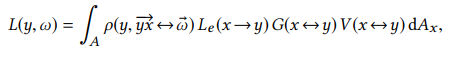
Where L is the outgoing radiance, ρ is the BSDF, Le is the emitted radiance , V is the visibility term, and G is the geometry term containing the attenuation and the cosine terms. Since computing an integral is prohibitively expensive, especially in real time, we generally try to form an estimator which tries to get as close to the true value as possible. Importance sampling estimates this integral by choosing N random samples from a source pdf to compute the following.

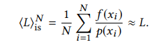
Ideally we have p(xi) proportional to f(xi) in order to reduce variance.

In reality however, due to the multiple terms in f(x), it is impossible to find a pdf that is perfectly proportional to the function, and this is where RIS comes in. The basic idea behing RIS is that we are going to approximate the function by finding a subobtimal pdf (called the source pdf) that is proportional to some of the terms in the function (for example the emitted radiance) and is easy to sample from. We then generate M candidate samples from this distrubution, and then randomly select an index z = {1,….., M} with probability as follows.

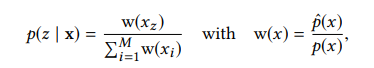
Where pˆ(x) is the target pdf for which no sampling pattern may exist (e.g., pˆ ∝ ρ · Le · G). A sample y is chosen and used to solve for the estimator;

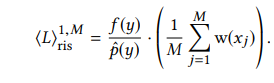
This can be intuitively be explained as the sample y was taken as if it was taken from the target pdf and the term in the parenthesis acts as a correction factor to account for the fact that it was in fact chosen from a suboptimal pdf. For N samples this estimator can be extended as;

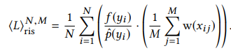
Weighted Reservoir Sampling (WRS)

Weighted reservoir sampling is a class of algorithms that allow the sampling of N random elements from a stream in a single pass. For a detailed explanation I highly recomment the WRS chapter in Raytracing Gems 2[1] but I will try to explain it in very simple terms here. Say we have a list of elements E and at a given time we are processing an element ‘i’ where 1 <= i <= N, from this list (the list for example could be light samples). Elements before ‘i’ were already processed and no are longer present in memory. WRS builds a very simple structure called a Reservoir which is a subset of the previously seen elements. As we go through the list of elements a random element ‘Ei’ is either chosen or discarded based on its relative weight;

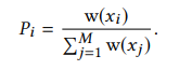
This may seem very familiar, because it is the exact same formula as the probability of choosing a random element from a pool of candidates derived from the source pdf in RIS. The paper [2] presents this pseudo code for the WRS algorithm.

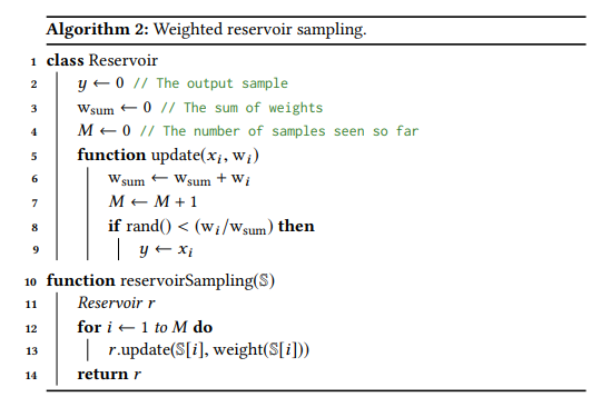
Here we can see a random number from [0…1] is compared with the relative weight of the element which is the ratio between the weight of the current element and the previously seen weights. We also maintain a variable M which counts the number of samples seen so far, and this will be used to calculate the final estimator. The current weight of the sample in our direct lighting case is the ratio between the source and the target pdf as described above.

Combining WRS and RIS

As I have implied before, it is very straightforward to apply the WRS algorithm to RIS to convert it to a streaming algorithm. The pseudo code from the paper describes it as follows.

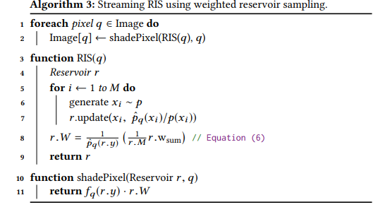
Here we are taking an M candidate samples and for each of them we are evaluating their source and target pdf to find their weight. We then use the sample, and the weight to update the reservoir as described in the previous section. This process is then repeated for all initial candidates, which in the case of direct lighting, can be a subset of the entire light list. In other words say we have N lights in the scene, we can choose an initial candidate count M, and then pick M random lights from the light list to update the reservoir with.

As we can see we have all the tools to convert RIS into a streaming algorithm and just doing this can provide excellent results to the lighting when compared to just stochastically sampling a light.

Spatiotemporal Reuse

Reservoirs also have an amazing property, they can be combined with other reservoirs without reprocessing the input streams. This is absolutely essential as it means that even when we might not have access to all the elements of a different stream, we can still combine its reservoir with another one to get a new reservoir. As the paper describes it, when combining reservoirs we consider the current sample y as a fresh sample with the weight wsum and feed it as an input to the new reservoir. This means that a new reservoir can be computed at constant time without having to store and retrieve all the input elements of the different reservoirs and only required reservoirs to be aware of their current state. The pseudo code for combining the reservoirs is as follows[2].

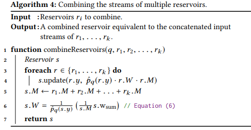
In the above algorithm, we are starting with an empty reservoir. Then, for each reservoir that we want to combine, we update the new reservoir with the current sample of the reservoir, and we weight it using the product of the probabalistic weight, the candidate count, and the target pdf at the current sample (which could be the magnitude of the lighting response of the current light sample). After this, the total number of candidates in the current reservoir is the sum of the total number of candidates seen by all the source reservoirs.

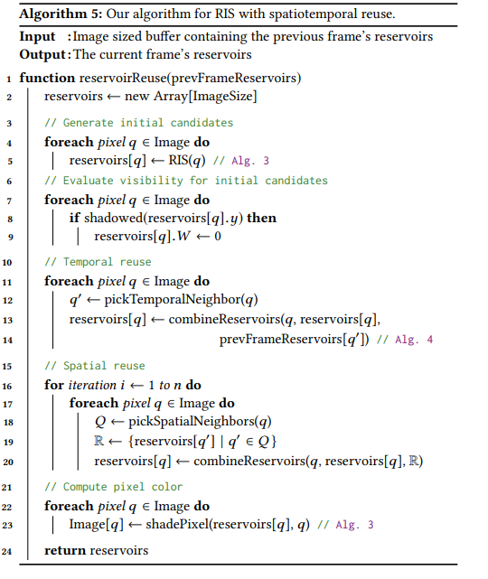
Since we not only have the reservoir for the current pixel, but also one for the neighboring pixels, we can combine their reservoirs to give a vastly better result than just using the current reservoir (this assumes that neighboring pixels are similar enough that they don’t add a lot of bias). Since images are usually rendered as a sequence of frames, especially in video games, we should also have access to the previous frame’s reservoir for the current pixel, and if that is the case we can combine those with the current reservior for temporal reuse. We also want to disregard samples that are occluded for a selected sample y for each pixel’s reservoir. We want to do this before the spatial and temporal reuse pass so that it doesn’t propagate to the neighboring pixels. The following pseudo code from the paper shows the entire algorithm and is by far the single most important thing to look at before implementing it in your own systems.

Implementation Details

In this section I will provide a very basic implementation of the above algorithm which should serve as a good starting point to implement something more robust. I implemented the algorithm in D3D12 using the DirectX Raytracing (DXR) API but the concepts should translate very well to any API.

I start by creating two screen space buffers, where each pixel contains a reservoir. My Reservoir structure is as follows, and I create two UAVs using this;

struct Reservoir
{
	float y; //The output sample
	float wsum; // the sum of weights
	float M; //the number of samples seen so far
	float W; //Probablistic weight
};

After this I modify my current direct lighting RayGen shaders (which are essentially DXR shaders which spawn the initial rays for raytracing against a scene BVH). First I generate M candidate samples from a list of point lights in my scene. I chose M = 32 as described by the paper since it produced optimal results for them.

     Reservoir reservoir = { 0,0,0,0};
        for (int i = 0; i < min(glightCount, 32); i++)
        {
            int lightToSample = min(int(nextRand(rndseed) * glightCount), glightCount - 1);
            Light light = lights.Load(lightToSample);
            float p = 1.0f / float(glightCount);

	    		// w of the light is f * Le * G / pdf   
            float3 brdfVal = PointLightPBRRaytrace(light, norm, pos, cameraPosition, roughness, metalColor.x, albedo, f0);
            
            float w = length(brdfVal) / p;
            UpdateResrvoir(reservoir, lightToSample, w, nextRand(rndseed));
            
            intermediateReservoir[launchIndex.y * WIDTH + launchIndex.x] = reservoir;

        }

Then I apply the temporal reuse pass using the previous frame’s reservoir. I use the motion vector to calculate where the current pixel was in the previous frame and use that value to index into the temporal reservoir buffer. I then combine the current reservoir with the temporal reservoir for the temporal resuse pass, and store it in the current frame’s reservoir for the spatial reuse pass. You can see my entire RayGen shader here

        //Temporal reuse
        Reservoir temporalRes = { 0, 0, 0, 0 };
        
        
        UpdateResrvoir(temporalRes, reservoir.y, p_hat * reservoir.W * reservoir.M, nextRand(rndseed));

        {
            Light light = lights.Load(prevReservoir.y);
            
            float L = saturate(normalize(light.position - pos));
            
            float ndotl = saturate(dot(norm.xyz, L)); // lambertian term

	    		// p_hat of the light is f * Le * G / pdf   
            float3 brdfVal = PointLightPBRRaytrace(light, norm, pos, cameraPosition, roughness, metalColor.x, albedo, f0);
            
            if (prevReservoir.M > 20 * reservoir.M)
            {
                prevReservoir.wsum *= 20 * reservoir.M / prevReservoir.M;
                prevReservoir.M = 20 * reservoir.M;
            }
            //prevReservoir.M = min(20.f * reservoir.M, prevReservoir.M); //As described in the paper, clamp the M value to 20*M
            float p_hat = length(brdfVal); // technically p_hat is divided by pdf, but point light pdf is 1
            UpdateResrvoir(temporalRes, prevReservoir.y, p_hat * prevReservoir.W * prevReservoir.M, nextRand(rndseed));

        }

For the spatial reuse pass I choose k = 5 neighboring samples randomly chosen from a 30 pixel radius. In order to reduce the bias from the spatial reuse the paper recommends to reject neighbors where the camera depth is greater than 10% of the current pixel or the angle between the current normal and neighbor’s normal is greater than 25 degrees. If the neighbor is acceptable we then combine it with the current reservoir to produce a new reservoir. I then repeat this step for all the neighbors. Once all the reservoirs have been combined into one. I calculate the lighting response with the current sample, and then weight it according to the RIS equation described in the theory section, which gives us the final lighting result.

  for (int i = 0; i < NUM_NEIGHBORS;i++)
    {        
        float radius = SAMPLE_RADIUS * nextRand(rndSeed);
        float angle = 2.0f * M_PI * nextRand(rndSeed);
        
        float2 neighborIndex = pixelPos;
        
        neighborIndex.x += radius * cos(angle);
        neighborIndex.y += radius * sin(angle);
         
        uint2 u_neighbor = uint2(neighborIndex);
        if (u_neighbor.x < 0 || u_neighbor.x >= WIDTH || u_neighbor.y < 0 || u_neighbor.y >= HEIGHT)
        {
            continue;
        }
        
        // The angle between normals of the current pixel to the neighboring pixel exceeds 25 degree		
        if ((dot(gBufferNorm[pixelPos].xyz, gBufferNorm[u_neighbor].xyz)) < 0.906)
        {
            continue;
        }
        
	//  Exceed 10% of current pixel's depth
        if (gBufferNorm[u_neighbor].w > 1.1 * gBufferNorm[pixelPos].w || gBufferNorm[u_neighbor].w < 0.9 * gBufferNorm[pixelPos].w)
        {
            continue;
        }
        
         Reservoir neighborRes = reservoirs[u_neighbor.y * uint(WIDTH) + u_neighbor.x];
         
        //Combine the neighborhood reservoir with the current reservoir
         
         lightSamplesCount += neighborRes.M;
    }
    
    reservoirNew.M = lightSamplesCount;

    //Adjusting the final weight of reservoir Equation 6 in paper
    Light light = lights.Load(reservoirNew.y);
    float L = saturate(normalize(light.position - pos));
            
    float ndotl = saturate(dot(norm.xyz, L)); // lambertian term

	    		// p_hat of the light is f * Le * G / pdf   
    float3 brdfVal = PointLightPBRRaytrace(light, norm, pos, camPos, roughness, metalColor.x, albedo, f0);
    float p_hat = length(brdfVal); // technically p_hat is divided by pdf, but point light pdf is 1
    
    if(p_hat == 0)
        reservoirNew.W == 0;
    
    else
        reservoirNew.W = (1.0 / max(p_hat, 0.00001)) * (reservoirNew.wsum / max(reservoirNew.M, 0.0001));
    
    outReservoir[pixelPos.y * uint(WIDTH) + pixelPos.x] = reservoirNew;
    
    outColor[pixelPos] = float4(brdfVal * reservoirNew.W, 1);

}

Closing Remarks and Future Work

These are the some screenshots for each step of the algorithm.

1. Stochastically selecting a light, no ReSTIR.

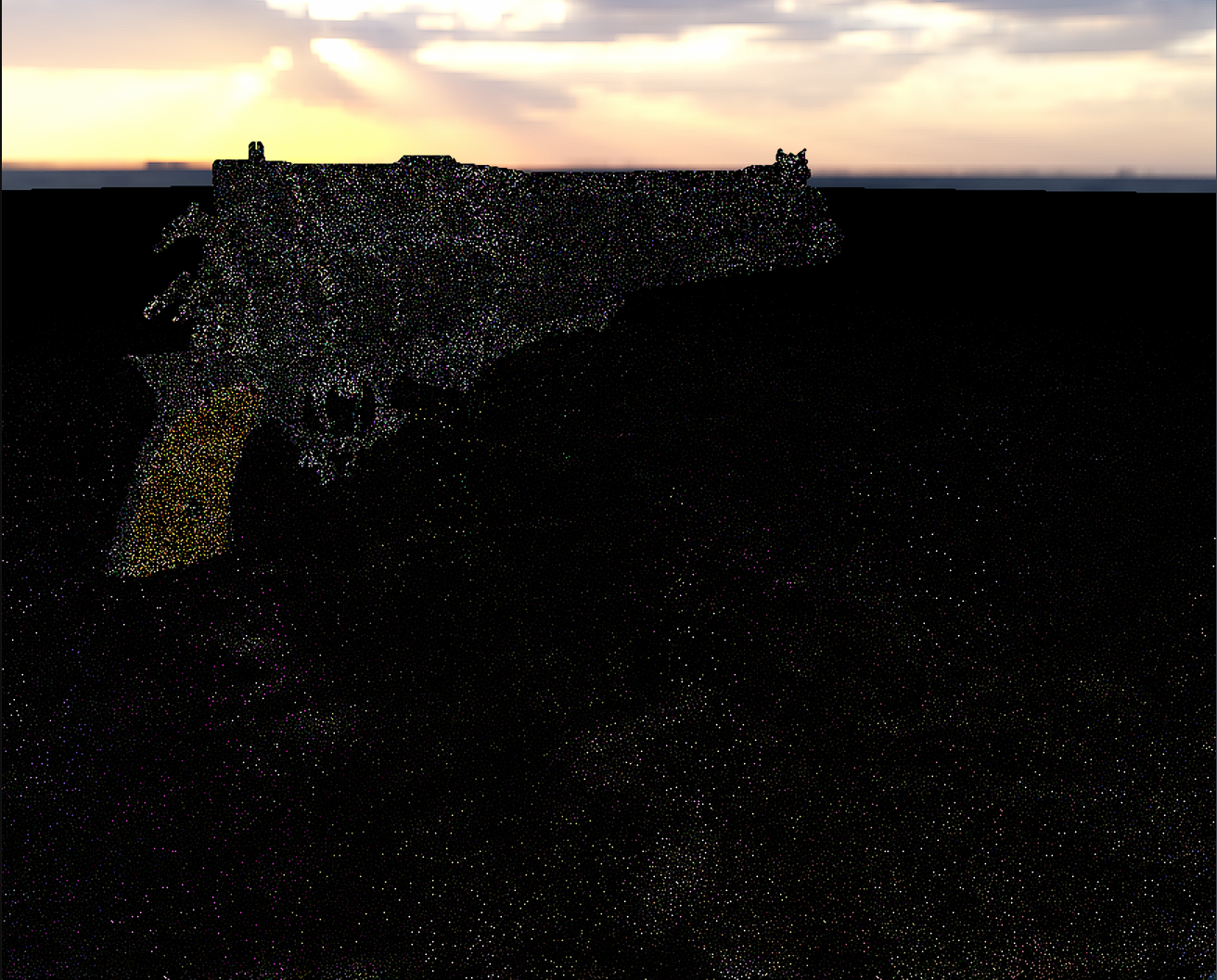
2. Temporal Reuse

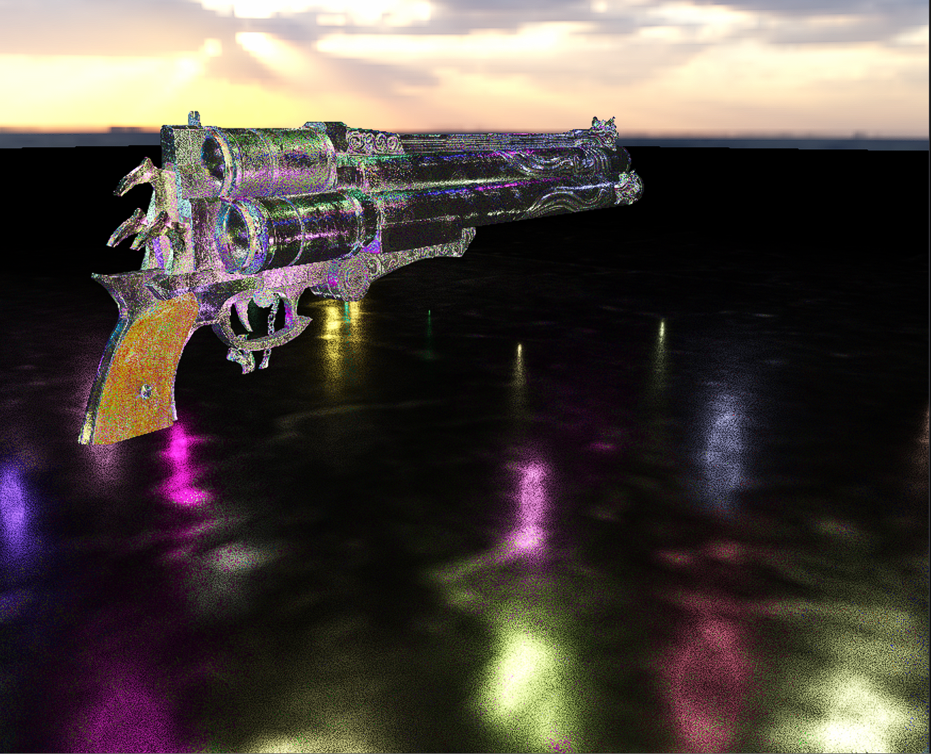
3. Spatial + Temporal Reuse

The spatiotemporal nature of the algorithm is very similar to how denoisers are structured which is one way to look at why the results are so dramatically better than just stochastically selecting a light from a list of 2000 point lights.

This algorithm has been extended for Global Illumination[3] called ReSTIR GI by Ouyang et. al. 2021, and I will explain the theory and implementation of that in a future post.

References

1. Raytracing Gems 2 Chapter on WRS
2. Original Paper for ReSTIR
3. ReSTIR GI Paper

Other ReSTIR samples that I found helpful

1)Falcor Implementation that extends the original algortithm for Indirect Diffuse Lighting

2)Vulkan Implementation of ReSTIR